Poisson regression
November 10, 2021
1. Insect communities in streams
The stream_composition.csv dataset shows the number of species of five insect orders in 20 streams, as a function of temperature and pH.
stream <- read.csv("stream_composition.csv")
str(stream)
## 'data.frame': 20 obs. of 8 variables:
## $ stream : int 1 2 3 4 5 6 7 8 9 10 ...
## $ pH : num 6.8 5.5 6.3 7.3 7.2 7 7 6.1 6.2 7.5 ...
## $ temperature: num 17.4 17.1 17 16.8 18.9 18.1 16.3 15 15.8 16.8 ...
## $ mayfly : int 26 17 7 17 27 28 19 6 9 19 ...
## $ stonefly : int 4 1 2 6 3 6 4 4 5 3 ...
## $ caddisfly : int 9 23 25 9 16 19 21 21 37 12 ...
## $ diptera : int 30 16 10 25 25 30 19 30 26 12 ...
## $ beetle : int 3 17 1 1 2 21 13 12 5 3 ...Estimate the effect of temperature and pH on the number of stonefly species, with a Poisson regression using the formula
stonefly ~ temperature + pH. Check if the data is overdispersed and correct your estimates if necessary.What portion of the variance in the number of species is explained by the model?
If one of the two variables has a significant effect, interpret the value of the coefficient.
Display the observed number of species and the fitted value curves for pH values ranging from 5.5 to 7.5 and for three temperature values: 15, 17 and 19 degrees C.
Hint: With ggplot, to ensure that prediction curves link points with the same value of a numeric variable (e.g. temperature), you must define a group (e.g. group = temperature) in the aes function. You could also convert the temperature to a factor.
Repeat steps (a) - (d) for a model of the number of mayfly species.
What is the mean number of mayfly species predicted by the model in (e) for a stream with a temperature of 17 degrees and a pH of 8.5? Is this prediction reliable?
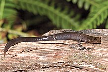
2. Salamanders in different forest landscapes
 Photo: Bill Bouton
The salamander.csv file contains data from Welsh and Lind (1995) on the number of salamanders (salaman) of species Plethodon elongatus in 47 plots (site), as a function of percentage forest cover (pct_cover) and forest age.
sal <- read.csv("salamander.csv")
str(sal)
## 'data.frame': 47 obs. of 4 variables:
## $ site : int 1 2 3 4 5 6 7 8 9 10 ...
## $ salaman : int 13 11 11 9 8 7 6 6 5 5 ...
## $ pct_cover : int 85 86 90 88 89 83 83 91 88 90 ...
## $ forest_age: int 316 88 548 64 43 368 200 71 42 551 ...From a Poisson regression, estimate the effect of forest cover on the number of salamanders per plot.
Does the
forest_agepredictor improve the predictive power of the model?Produce a graph of the number of salamanders according to forest age and superimpose points representing the fitted values for the model based solely on forest cover. What do you observe?
Based on these results, do you think that the forest age directly influences the salamander population? Does it indirectly influence this population?