Why R?

What is R?

R refers both to a programming language and to the software that interprets commands written in that language.
The language was originally developed for statistical analysis.
A large number of packages add to the basic features of R.
R is distributed as free software (open source).

Why write programs for data analysis?

Why should you write programs (or scripts) to perform data analyses, rather than using graphical interface software (such as Excel)? Learning a language like R requires more time initially, but brings several benefits.

The scripts are a faithful record of the analyses performed on a dataset. You, your collaborators or other researchers will easily be able to replicate this analysis in the future (e.g. when new data is available).
Scripts automate repetitive tasks (e.g. perform the same analysis on 100 data files).

Why program in R?

Functions and basic data types are designed for statistics.
Free access to the software facilitates the sharing of programs between researchers.
Many modules exist for specialized analyses in different fields, including ecology.
Given the large community of users, it is easy to find help online.

RStudio

The RStudio software is a programming environment (IDE) with several features that simplify the interactive use of the R language.
By default, the RStudio window is divided into 4 sections. We will first use the console (lower left corner).

Objectives for this part

Discover the basic functions of the R language.
Become familiar with the RStudio interface.
Know the main data types (numeric, character, and logical values) and data structures (vector, list, matrix, data frame) in R.
Load a data frame from an external file.
Subset a data structure.
Write your own functions.

Basic operations in R

R as a calculator

The > symbol in the console indicates that R is ready to receive a command. R includes basic arithmetic operations: +, -,*,/and^(power).

(4 + 3) * 2

## [1] 14

5 ^ 3

## [1] 125

Question: Why is the result preceded by [1]?

Answer: R indicates that this is the first element of the result. In this case, there is only one element.

Comparison operators

We use == to check if two expressions are equal and != to see if they are different. R also recognizes the comparisons <, <=, > and >=.

(4 + 3) * 2 != 4 + (3 * 2)

## [1] TRUE

Mathematical functions

Several mathematical functions are defined in R, such as exp,log, sqrt (square root), as well as trigonometric functions and constants like pi.

cos(pi)

## [1] -1

Exercise 1

After replacing $x$ with a number of your choice, transcribe the following proposition in R and check that it returns TRUE:

\[(\sin x)^2 + (\cos x)^2 = 1\]

Solution

Calling functions

Note that parentheses () play two roles in R:

They delimit parts of a mathematical expression (e.g. (4 + 3) * 2).
They follow the name of a function and contain the arguments of that function. If there are multiple arguments, they are separated by commas.

For example, the seq(a, b) function creates a sequence of integers between a andb:

seq(1, 50)

##  [1]  1  2  3  4  5  6  7  8  9 10 11 12 13 14 15 16 17 18 19 20 21 22 23 24 25
## [26] 26 27 28 29 30 31 32 33 34 35 36 37 38 39 40 41 42 43 44 45 46 47 48 49 50

Create a variable

The <- operator is used to assign the value of an expression to a variable. If the variable does not exist, it is created by R at this time.

x <- 5:10

Note that the : operator is a shortcut for the seq(5, 10) statement.

Tip: To save some time in RStudio, the keyboard shortcut Alt + - produces the <- operator.

To find the value of a variable, just enter its name:

## [1]  5  6  7  8  9 10

Also note that the x variable appeared in the Environment tab (upper right corner) in RStudio. This tab allows you to quickly consult all variables currently in memory.

Rules for naming objects in R

In R, the name of an object recognized by the software (variable, function, etc.) must begin with a letter and may include letters, numbers, or the characters _ and .. Note that R is case-sensitive.

## Error in eval(expr, envir, enclos): objet 'X' introuvable

Tips:

To make the code more readable, object names must (while still being brief) provide information about their contents. For example, diametre ordiam rather than d orx.

It is better to adopt a uniform style for object names. We recommend using only lowercase letters and separating compound names with _, e.g. temp_min for minimum temperature.

Character strings

To represent textual data, we use strings of characters, which must be enclosed in quotation marks to differentiate them from the commands and objects of the code.

s <- "text"

Note: Single quotation marks (’) are also accepted by R, but we will only use double quotation marks for consistency.

Get help

The documentation of a function can be found by preceding its name with a question mark, e.g. ?seq. In RStudio, the help page appears on the Help tab (lower right corner). If you do not know the exact name of the function, use two question marks, e.g. ??logarithm. You can also write directly in the search window of the Help tab.

Many websites offer information about R. Often, the fastest way to get help for a specific problem is to write your question in a search engine.

Vectors and data types

Vector properties

The variable x that we created earlier is a vector with 6 elements (the numbers 5 to 10). The vector is the simplest data structure in R; a variable comprising a single element is in fact a vector of length 1. All the elements of a vector must be of the same type of data. We can determine the length of a vector with the function length, and its type with theclass function.

length(x)

## [1] 6

class(x)

## [1] "integer"

Editor in RStudio

Until now, we have entered commands directly into the console. To save a list of commands, which will eventually become an analysis script, we will use the editor in RStudio (upper left corner).

Note: When you open a new session on RStudio, an empty script should appear in the editor. If not, go to File -> New File -> R Script to create a new script.

Create a vector

The c function combines several values into a vector.

Enter the following commands in the editor, then execute them with the Run button (top right of the editor) or with the keyboard shortcut Ctrl + Enter. In both cases, the cursor must be placed on the line to be executed. You can also select a block of lines to execute at once.

# Diameter in cm and species of three trees
diam <- c (7.5, 3, 1.4)
species <- c ("fir", "pine", "birch")

Comment lines

Lines starting with # are never executed by R. These are comments that add context and clarify the purpose of a section of the code.

Exercise 2

What is the data type of the vector species?
What happens if you try to create a vector with different types of data, e.g.: c (1, 2, "pine")?

Solution

Vector operations

In R, basic mathematical operations are vectorized, that is, they apply separately to each element of a vector.

v <- c(1, 4, 9)
sqrt(v)

## [1] 1 2 3

v + c(10, 20, 30)

## [1] 11 24 39

If the two vectors do not have the same number of elements, the shortest vector is “recycled”; this is especially useful for operations involving a vector and a single value.

diam10 <- diam * 10
diam10

## [1] 75 30 14

esp_pin <- species == "pine"
esp_pin

## [1] FALSE  TRUE FALSE

Note that the esp_pin variable is of logical type (true / false).

Summary of basic data types

integer
numeric (real numbers, also calleddouble)
character (strings)
logical (possible valuesTRUE or FALSE, always in uppercase letters)

Data frames

A data frame is a two-dimensional data structure formed by combining vectors of the same size. It is used to represent a series of observations (rows) of the same set of variables (columns).

trees <- data.frame(species, diam)
trees

##   species diam
## 1     fir  7.5
## 2    pine  3.0
## 3   birch  1.4

The str() function provides more details about the structure of an object.

str(trees)

## 'data.frame':    3 obs. of  2 variables:
##  $ species: chr  "fir" "pine" "birch"
##  $ diam   : num  7.5 3 1.4

Load a data frame from a file

Most of the time, we want to load tables of existing data rather than create them in R. We will see here how to import data saved in CSV format (comma-separated values).

First, make sure that R points to the right working directory. In the Files tab (lower right corner of RStudio), use the “…” button on the right to navigate to the directory containing the data file cours1_kejimkujik.csv, then click on More -> Set As Working Directory. (You can also call the setwd function in R with a path to the directory.) The current working directory is displayed on the line at the top of the console.

Next, call the read.csv function to load tree inventory data from plots in the Kejimkujik National Park, Nova Scotia:

kejim <- read.csv("cours1_kejimkujik.csv")
str(kejim)

## 'data.frame':    1161 obs. of  9 variables:
##  $ site     : chr  "BD" "BD" "BD" "BD" ...
##  $ parcelle : chr  "A" "A" "A" "A" ...
##  $ jour     : int  31 31 31 31 31 31 31 31 31 31 ...
##  $ mois     : int  8 8 8 8 8 8 8 8 8 8 ...
##  $ annee    : int  2004 2004 2004 2004 2004 2004 2004 2004 2004 2004 ...
##  $ num_arbre: int  1 2 6 7 8 9 10 11 12 13 ...
##  $ nb_tiges : int  1 1 1 1 1 1 1 1 1 1 ...
##  $ espece   : chr  "TSCA" "TSCA" "TSCA" "ACRU" ...
##  $ dhp      : num  16.3 24 29.8 29 15.5 32 11.3 44.8 17.2 70.5 ...

Tips

The Tab key gives access to several types of help in RStudio, depending on the context. For example, we can get:

a list of functions beginning with a combination of letters already entered;

the possible arguments for the function (if the cursor is between the parentheses);

the list of files in the working directory (if the cursor is enclosed in quotation marks).

The French version of software like Excel uses the comma as a decimal sign, and produces CSV files with the semicolon as a field separator. For this type of file, replace read.csv withread.csv2.

The head function shows the first rows (by default, the first 6) of a data frame.

head(kejim)

##   site parcelle jour mois annee num_arbre nb_tiges espece  dhp
## 1   BD        A   31    8  2004         1        1   TSCA 16.3
## 2   BD        A   31    8  2004         2        1   TSCA 24.0
## 3   BD        A   31    8  2004         6        1   TSCA 29.8
## 4   BD        A   31    8  2004         7        1   ACRU 29.0
## 5   BD        A   31    8  2004         8        1   TSCA 15.5
## 6   BD        A   31    8  2004         9        1   TSCA 32.0

The dim function gives the dimensions (rows, columns) of the data frame. These dimensions can also be obtained separately with nrow andncol.

dim(kejim)

## [1] 1161    9

Select elements of a vector or a data frame

Extract a variable from a data frame

In R, the $ operator allows to extract a part of a complex object, and in particular, to extract a variable (column) from a data frame.

dhp <- kejim$dhp

Here, the result dhp is a numeric vector.

Extract elements from a vector

To extract certain elements of a vector according to their position, we use the brackets ([]):

dhp[2]

## [1] 24

dhp5 <- dhp[1:5]
dhp5

## [1] 16.3 24.0 29.8 29.0 15.5

In the second case, we gave a vector of indices to extract the first 5 values of dhp.

With negative integers, we can exclude values based on their position:

dhp5[-2]

## [1] 16.3 29.8 29.0 15.5

Finally, it is possible to select values according to a logical condition. In the statement below, R determines the positions of the TRUE values in the dhp5 > 20 logical vector, and then extracts the values of dhp5 corresponding to those positions:

dhp5[dhp5 > 20]

## [1] 24.0 29.8 29.0

To replace specific elements in a vector (or in a data frame column), we combine selection and assignment. The code below replaces the DHP values smaller than 1 with the value 1.

dhp[dhp < 1] <- 1

Exercise 3

What does the following command mean?

esp_dhp50 <- kejim$espece[kejim$dhp > 50]

Create a vector with DHP measurements for all trees with more than one stem (nb_tiges variable).

Solution

Extract a section from a data frame

You can also use the [] notation to extract part of a data frame. In this case, the subsets of rows and columns are separated by a comma:

kejim[1:5, 6:9]

##   num_arbre nb_tiges espece  dhp
## 1         1        1   TSCA 16.3
## 2         2        1   TSCA 24.0
## 3         6        1   TSCA 29.8
## 4         7        1   ACRU 29.0
## 5         8        1   TSCA 15.5

You can also select columns with a vector of names:

kejim2 <- kejim[, c("num_arbre", "espece", "dhp")]
str(kejim2)

## 'data.frame':    1161 obs. of  3 variables:
##  $ num_arbre: int  1 2 6 7 8 9 10 11 12 13 ...
##  $ espece   : chr  "TSCA" "TSCA" "TSCA" "ACRU" ...
##  $ dhp      : num  16.3 24 29.8 29 15.5 32 11.3 44.8 17.2 70.5 ...

Note:

The absence of information before the comma means that we want to keep all the rows.
The names of columns are in quotation marks here, unlike when you extract a single column with $.

Base graphics

R contains some basic functions to visualize data. In the example below, the plot function displays the values in a vector in order of their position (index), and the hist function shows a histogram of these values.

plot(kejim$dhp)
plot(kejim$dhp)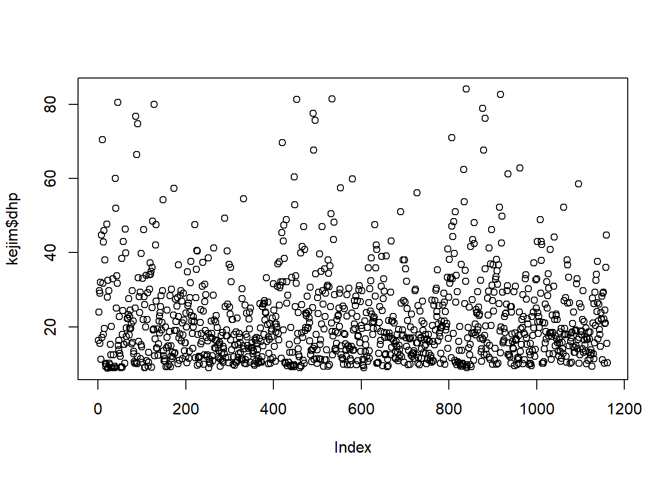

Other data structures

Matrix

A matrix is a two-dimensional data structure where all elements have the same type. It can be created with the matrix function.

mat1 <- matrix(1:12, nrow = 3)
mat1

##      [,1] [,2] [,3] [,4]
## [1,]    1    4    7   10
## [2,]    2    5    8   11
## [3,]    3    6    9   12

As for a data frame, we extract the elements of a matrix by specifying two vectors of indices:

mat1[2, 3]

## [1] 8

mat1[1:2, 2:3]

##      [,1] [,2]
## [1,]    4    7
## [2,]    5    8

List

Unlike a vector, a list can contain objects of different types. We create a list with the list function and we extract individual elements using double brackets[[ ]].

list1 <- list(1, 2, "ab")
list1

## [[1]]
## [1] 1
## 
## [[2]]
## [1] 2
## 
## [[3]]
## [1] "ab"

list1[[3]]

## [1] "ab"

A list can even contain vectors or other lists:

list2 <- list(c(10, 20), "cd", list1)
str(list2)

## List of 3
##  $ : num [1:2] 10 20
##  $ : chr "cd"
##  $ :List of 3
##   ..$ : num 1
##   ..$ : num 2
##   ..$ : chr "ab"

We will not discuss these structures in more detail for the moment. In summary, the four data structures we have seen are differentiated according to whether they have 1 or 2 dimensions and whether they contain elements of the same type or of different types.

	Same type	Different types
1D	vector	list
2D	matrix	data frame

Other useful functions

sort: Orders a vector in ascending order.

sort(dhp5)

## [1] 15.5 16.3 24.0 29.0 29.8

sum: Calculates the sum of the values of a vector.

sum(kejim$nb_tiges)

## [1] 1190

summary: Returns the minimum, maximum, average and quartiles of a numeric variable.

summary(kejim$dhp)

##    Min. 1st Qu.  Median    Mean 3rd Qu.    Max. 
##    8.80   13.00   18.40   21.76   26.50   84.10

table: Counts the number of occurrences of each value of a vector (useful for categorical or discrete values).

table(kejim$espece)

## 
## ABBA ACPE ACRU BEAL BECO BEPA FAGR PIRU PIST POGR POTR QURU TSCA 
##   27    4  246    9   18  117   39  109  131   45    3   64  349

With two or more vectors, table creates a contingency table:

table(kejim$espece, kejim$site)

##       
##         BD CFR  CL CLT NCL  PL
##   ABBA   3   0  10  11   0   3
##   ACPE   0   4   0   0   0   0
##   ACRU  23   2  52  82  25  62
##   BEAL   0   0   9   0   0   0
##   BECO   0   0  18   0   0   0
##   BEPA   0   9   0  40  36  32
##   FAGR   0  17  22   0   0   0
##   PIRU  12  67   0   3  27   0
##   PIST   3   2   3  40   9  74
##   POGR   0   0   0   0  19  26
##   POTR   0   0   0   3   0   0
##   QURU   0   3   0  26   0  35
##   TSCA  90  36   0   0 165  58

There are also several functions for calculating different statistics from a data vector: mean,median min,max, sd (standard deviation).

Exercise 4

In R, the logical values TRUE and FALSE correspond to numerical values 1 and 0, respectively.

How do you interpret the result of sum(c(FALSE, TRUE, TRUE))?
How can you use the sum function to determine the number of red maples (species code “ACRU”) in the kejim data?

Solution

Missing values

To represent missing data, R uses the NA symbol (in uppercase and without quotation marks). Generally, the result of any calculation involving a NA value is also NA. Some functions like sum andmean have a na.rm argument to ignore missing values.

v_na <- c (1, 2, 9, NA)
mean(v_na)

## [1] NA

mean(v_na, na.rm = TRUE)

## [1] 4

Write your own functions

As mentioned above, one of the advantages of a programming language like R is the ability to automate repetitive operations through functions. Thus, you can define your own functions, in order to create a “shortcut” to a sequence of simpler operations.

Here is the basic structure of an R function:

name_of_function <- function (argument1, argument2, ...) {
    # enter the function code here
}

By default, the result of the function is that obtained by the last instruction of the function block (block delimited by the braces {}).

As an example, we will create a tree_type function that will indicate whether a species found in the kejim dataset is a conifer or a broadleaf tree.

# Indicates whether the tree species is a conifer or broadleaf tree
tree_type <- function (species) {
    # code to write ...
}

First, we need a vector of species codes corresponding to conifers. In this dataset, there are four: balsam fir (ABBA), red spruce (PIRU), white pine (PIST) and eastern hemlock (TSCA).

codes_conif <- c ("ABBA", "PIRU", "PIST", "TSCA")

Then we will use the %in% function included in R, which tests whether the elements of a vector are found in another vector. For example:

"TSCA" %in% codes_conif

## [1] TRUE

Finally, we need to output a different result depending on the result of the logical test. This is used for the if .. else ... branch, which takes the following form:

if (condition) {
    # code to execute if condition is true
} else {
    # code to execute if condition is false
}

Here is our finalized function:

# Indicates whether the tree species is a conifer or broadleaf tree
tree_type <- function (species) {
    codes_conif <- c ("ABBA", "PIRU", "PIST", "TSCA")
    if (species %in% codes_conif) {
        type <- "conifer"
    } else {
        type <- "broadleaf"
    }
    type
}

Note that the statements in a block of code (that of the function, as well as the blocks if andelse) are indented (offset). An indentation of at least 4 characters is recommended to facilitate understanding of the logic of the code.

The result of the function corresponds to that of the last instruction, so here it will be the content of the variable type.

tree_type("ACRU")

## [1] "broadleaf"

tree_type("PIST")

## [1] "conifer"

Review

Functions and essential operations

Operator	Usage
`?`	Get help on a function
`#`	Add a comment
`:`	Define a sequence of integers
`<-`	Assign a value to an object
`$`, `[]`, `[[]]`	Select part of an object
`" "`	Delimit strings
`{}`	Delimit a block of code (e.g. function)
`+`, `-`, `*`, `/`, `^`	Arithmetic operators
`==`, `! =`, `<`, `>`, `<=`, `>=`	Comparison Operators
`%in%`	Inclusion operator

Function	Usage
`c()`	Create a vector
`class()`	Class (type) of an object
`str()`	Structure of an object
`length()`	Length of a one-dimensional object
`dim()`	Dimensions of an object
`head()`	See the first rows of a table
`summary()`	Summary of a numeric vector
`table()`	Number of occurrences of values in a vector

Select elements of an object

Here, i, j, k and l are positive integers, while condition is an expression that returns TRUE or FALSE.

Expression	Result
`v[c(i, j)]`	The elements of the vector v in position i and j.
`v[-c(i, j)]`	The elements of v except those in position i and j.
`v[condition]`	The elements of v for which condition is true.
`df$name`	The vector corresponding to the column name of the table df.
`df[c(i, j), c(k, l)]`	The elements in one of the rows i or j and in one of the columns k or l of df (also works for a matrix).
`df[condition, ]`	The rows of df for which condition is true.
`df [i:j, c("name1", "name2")]`	The elements in columns name1 and name2 are in rows from i to j.

References

The content of this part is based on an introductory course in R prepared by Marc Mazerolle (professor at U. Laval, formerly UQAT), as well as a workshop offered by the Socio-Environmental Synthesis Center (SESYNC) and available online at: https://cyberhelp.sesync.org/basic-R-lesson/.

Exercise solutions

Exercise 1

For example, with $x$ = 1.5

sin(1.5)^2 + cos(1.5)^2 == 1

## [1] TRUE

Back

Exercise 2

class(species)

## [1] "character"

c(1, 2, "pine")

## [1] "1"    "2"    "pine"

The vector c(1, 2,"pine") is of type character because numbers can be represented as text, but text cannot be represented as numbers.

Back

Exercise 3

esp_dhp50 is a vector of species corresponding to trees in kejim with DHP greater than 50 cm.

dhp_multi_tige <- kejim$dhp[kejim$nb_tiges > 1]

Back

Exercise 4

The sum of a logical vector is the number of true values.

sum(kejim$espece == "ACRU")

## [1] 246

Back

Introduction to R - Part 1

September 1, 2021

Why R?

What is R?

Why write programs for data analysis?

Why program in R?

RStudio

Objectives for this part

Basic operations in R

R as a calculator

Comparison operators

Mathematical functions

Exercise 1

Calling functions

Create a variable

Rules for naming objects in R

Character strings

Get help

Vectors and data types

Vector properties

Editor in RStudio

Create a vector

Comment lines

Exercise 2

Vector operations

Summary of basic data types

Data frames

Load a data frame from a file

Select elements of a vector or a data frame

Extract a variable from a data frame

Extract elements from a vector

Exercise 3

Extract a section from a data frame

Base graphics

Other data structures

Matrix

List

Other useful functions

Exercise 4

Missing values

Write your own functions

Review

Functions and essential operations

Select elements of an object

References

Exercise solutions

Exercise 1

Exercise 2

Exercise 3

Exercise 4