Course synthesis
Sampling and experiment design
Sampling
- Simple random sampling: each individual has the same probability of being sampled
- Systematic sampling: regularly-spaced samples from a random origin
- Stratified sampling: division of population into strata, random sampling by stratum
- Cluster sampling: sample groups of individuals, take either all the individuals of a group, or a simple random sample by group (multistage)
Experimental design
- Control group
- Random assignment of individuals to treatments
- Control of variation using blocks
- Split plots: second factor varies within replicates of the first factor
Structure of a statistical test
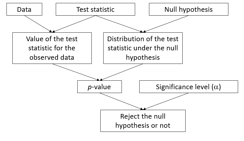
Examples
| One-sample \(t\)-test (\(n\) individuals) | One-factor ANOVA (\(m\) groups of \(n\) individuals) | |
|---|---|---|
| Null hypothesis | The mean \(\bar{x}\) equals \(\mu\) | Same mean in each of the \(m\) groups |
| Statistic | \(t = (\bar{x} - \mu) / (s/\sqrt{n})\) | \(F = MSA/MSE\) |
| Distribution | \(t\) with \(n-1\) degrees of freedom | \(F\) with \(m(n-1)\) and \((m - 1)\) degrees of freedom |
Key points for hypothesis testing
The significance level is the probability of rejecting the null hypothesis when it is true.
You must choose a test and a significance level before analyzing the results.
If several tests are performed in an experiment, the probability of mistakenly rejecting one of the null hypotheses increases (multiple comparison problem).
The power of a test is the probability of rejecting the null hypothesis if it is false. The smaller the effect to be detected compared to the variance of the response (low signal-to-noise ratio), the higher \(n\) must be to have the same power.
With a sufficiently large \(n\), even a very small effect will be judged statistically significant; it does not mean that the effect is important.
Parameter estimation
Bias: systematic difference between the estimate of a parameter and its exact value.
Standard error: standard deviation of the estimate of a parameter due to limited sampling; decreases when \(n\) increases.
- Different from the standard deviation of the response: measures the variability between individuals, does not depend on \(n\).
Confidence interval: In X% of the possible samples, the X% confidence interval of a parameter estimate contains the true value of this parameter.
Relationship between confidence interval and hypothesis testing: the hypothesis \(\theta = \theta_0\) can be rejected at a threshold \(\alpha\) if the \(100 \% (1 - \ alpha)\) confidence interval of \(\hat{\theta}\) does not include \(\theta_0\).
Test differences between groups
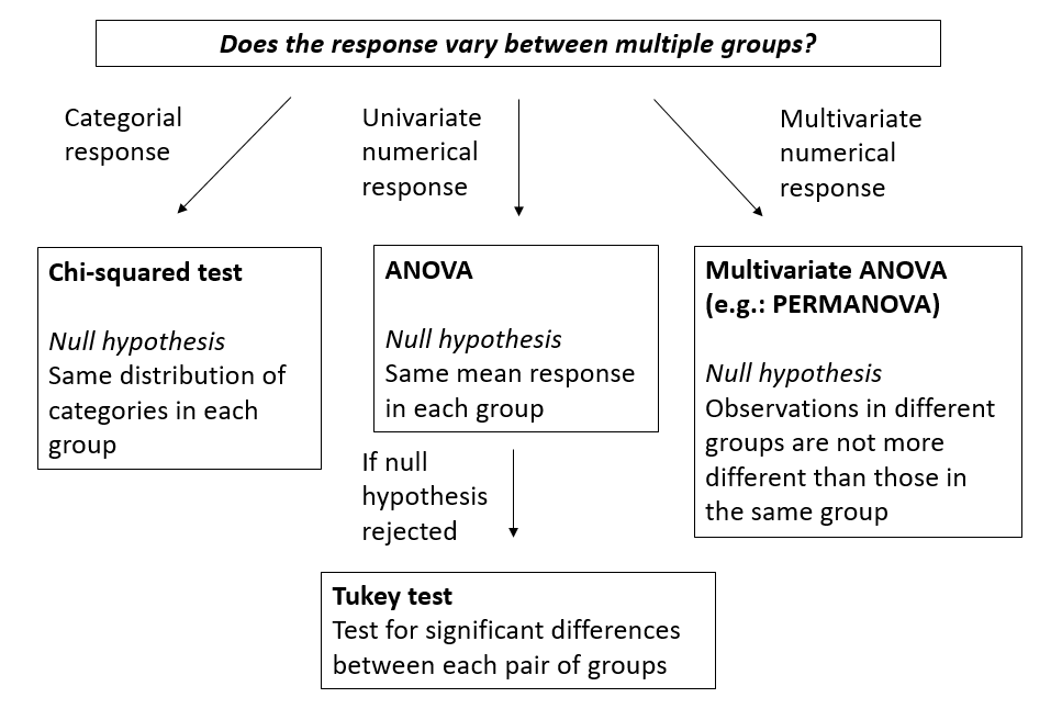
Assumptions of the ANOVA
- Independence: The observations are independent.
- Normality: The response follows a normal distribution in each group.
- Homoscedasticity: The variance is the same in each group.
ANOVA tolerates moderate deviations from normality, so that assumption is less critical than the other two.
With only 2 groups, the \(t\)-test allows for unequal variances.
Regression models
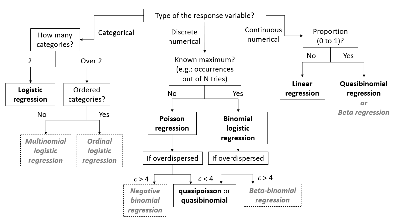
Models in gray not seen in this course.
Assumptions of the linear regression model
- Linear and additive effect of predictors on response
- Otherwise: transform the response and / or predictors, include interactions, generalized additive models (GAM)
- Independence of residuals
- Otherwise: mixed models (grouped data), temporal or spatial autocorrelation models
- Uniformity of the variance (homoscedasticity)
- Otherwise: transform the response, weighted linear regression
- Normality
- Otherwise: transform the response (only if very far from normality)
Model names in italics not seen in this course.
Interpreting regression coefficients
Linear regression, no interactions
\[ y \sim w + x + z \]
\(y\) is the numerical response, \(w\) and \(x\) are numerical predictors, \(z\) is a factor with treatment coding (default in R) and three levels: A (reference), B, and C.
Estimated coefficients:
- (Intercept): Mean value of the response when all predictors are at their reference level (0 for numerical predictors).
- w: Effect on \(y\) of a unit increase of \(w\) if \(x\) and \(z\) remain constant.
- x: Effect on \(y\) of a unit increase of \(x\) if \(w\) and \(z\) remain constant.
- zB: Difference of \(y\) between levels B and A of \(z\), if \(w\) and \(x\) remain constant.
- zC: Difference of \(y\) between levels C and A of \(z\), if \(w\) and \(x\) remain constant.
Interaction of a numerical predictor and a factor
\[ y \sim x * z \]
Estimated coefficients:
- (Intercept): Same interpretation.
- x: Effect on \(y\) of a unit increase of \(x\) if \(z\) = A.
- zB: Difference of \(y\) between levels B and A of \(z\) if \(x\) = 0.
- zC: Difference of \(y\) between levels C and A of \(z\) if \(x\) = 0.
- x:zB: Difference between the slope of \(y\) vs. \(x\) if \(z\) = B and that slope if \(z\) = A.
- x:zC: Difference between the slope of \(y\) vs. \(x\) if \(z\) = C and that slope if \(z\) = A.
In other words, to get the slope of \(y\) vs. \(x\) if \(z\) = B, we must add the coefficients x and x:zB.
Interaction of two numerical predictors
\[ y \sim w * x \]
Estimated coefficients:
- (Intercept): Same interpretation.
- w: Effect on \(y\) of a unit increase of \(w\) if \(x\) = 0.
- x: Effect on \(y\) of a unit increase of \(x\) if \(w\) = 0.
- w:x: Effect on the slope of \(y\) vs. \(x\) of a unit increase in \(w\), OR effect on the slope of \(y\) vs. \(w\) of a unit increase in \(x\) (two equivalent interpretations).
Generalized linear models
In these models, the mean of \(y\) is not equal to the linear combination of predictors \(\eta\), but to a transformation of \(\eta\) according to a link function.
The interpretation of the parameters above indicates the effect on \(\eta\). To obtain the effect on the mean of \(y\), you must apply the inverse of the link function.
- Inverse of the logit link: \(y = 1/(1 + \exp(- \eta))\)
- Inverse of the log link: \(y = \exp(\eta)\)
Standardization of numerical predictors
- Standardize a predictor by subtracting the mean and dividing by the standard deviation.
\[ x_{norm} = \frac{x - \mu_x}{\sigma_x} \] - Since \(x_{norm} = 0\) corresponds to the mean of \(x\), it is easier to interpret the intercept in all cases, and the coefficients in the case of a model with interactions.
- Since a unit increase of \(x_{norm}\) corresponds to increasing \(x\) by one standard deviation, the magnitude of the coefficient gives an idea of the importance of the effect of this predictor. We can thus compare predictors with different original scales.
Model selection
Choice between models of different complexities: compromise between underfitting and overfitting.
Underfitting: important effects not included in the model.
Overfitting: the model reproduces very well the data used to fit it, but performs worse on new data.
In the absence of independent data to evaluate the predictive power of different models, we can estimate it with the AIC (and its variants).
Key points for model selection
Compare models based on the same response variable and the same observations.
The best model may not be good: check the fit.
If several models are plausible, the weighted average of their predictions is often better than the predictions of the best model.
Collinearity
Problem where two or more predictors are strongly correlated.
Different options:
- Choose a priori which predictors to eliminate, according to our knowledge of the system.
- Use AIC to choose between different models that include non-collinear subsets of predictors.
- Perform an ordination of the predictors to obtain uncorrelated axes, then perform a regression the response according to these new variables.