The bootstrap method

Data

For this lab, we will use the dataset sphagnum_cover.csv, from the paper:

Maanavilja, L., Kangas, L., Mehtätalo, L. and Tuittila, E.‐S. (2015), Rewetting of drained boreal spruce swamp forests results in rapid recovery of Sphagnum production. J Appl Ecol, 52: 1355-1363. doi:10.1111/1365-2664.12474)

This dataset contains measurements of the percentage cover of sphagnum moss (sphcover) for 36 boreal swamps divided into three types (habitat): Dr = drained, Re = rewetted et Un = undrained.

cover <- read.csv("sphagnum_cover.csv")
str(cover)

## 'data.frame':    36 obs. of  3 variables:
##  $ site    : chr  "AmLuxx" "EvLuPa" "EvLuVK" "HeLuxx" ...
##  $ habitat : chr  "Un" "Un" "Un" "Un" ...
##  $ sphcover: num  35.3 56.2 46.6 56 54.3 ...

1. Estimation of mean cover for drained swamps

From the dataset, extract the sphcover values for drained swamps. Calculate the mean percentage cover and its standard error from the usual formula (based on standard deviation and sample size). Finally, calculate the 95% confidence interval based on the $t$ distribution:

\[(\bar{x} + t_{(n-1)0.025} s_{\bar{x}}, \bar{x} + t_{(n-1)0.975} s_{\bar{x}})\]

Reminder: The function qt(p, df) gives the quantile corresponding to a given cumulative probability p, for a $t$ distribution with df degrees of freedom.

Solution

cov_dr <- cover$sphcover[cover$habitat == "Dr"]

n <- length(cov_dr)

# Mean
moy <- mean(cov_dr)
moy

## [1] 7.16229

# Standard error
err_type <- sd(cov_dr) / sqrt(n)
err_type

## [1] 2.517416

# Confidence interval
ic <- c(moy + qt(0.025, n - 1) * err_type, 
        moy + qt(0.975, n - 1) * err_type)
ic

## [1]  1.357118 12.967461

Simulate 10,000 bootstrap samples for the mean calculated in a). What is its standard error according to the bootstrap? Does this statistic appear biased?

Solution

library(boot)
set.seed(5612)

calc_moy <- function(x, i) mean(x[i])

boot_moy <- boot(cov_dr, calc_moy, R = 10000)

# Erreur-type
sd(boot_moy$t)

## [1] 2.386784

# Biais
mean(boot_moy$t) - boot_moy$t0

## [1] 0.0328031

The bias is quite small (compared to the standard error) and could be due to a numerical error rather than a real bias in the statistic.

How does the bootstrap distribution differ from a normal distribution? To answer this question, it may be useful to draw a quantile-quantile plot (in the code below, res is the result of the bootstrap):

qqnorm(res$t)
qqline(res$t)

Solution

qqnorm(boot_moy$t)
qqline(boot_moy$t)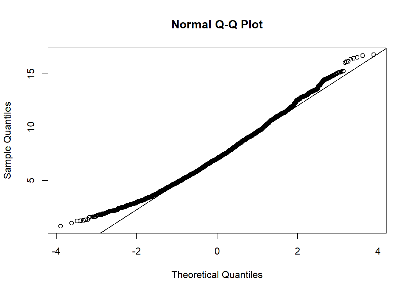

The bootstrap distribution is skewed: the smallest values are above the line, therefore closer to the mean compared to a normal distribution, while the largest values are also above the line, therefore further from the mean.

Calculate the 95% confidence interval of the mean using the BCa method. How does it differ from the one calculated in a) using the classical formula? Can you explain this difference based on the result in c)?

Solution

boot.ci(boot_moy)

## Warning in boot.ci(boot_moy): bootstrap variances needed for studentized
## intervals

## BOOTSTRAP CONFIDENCE INTERVAL CALCULATIONS
## Based on 10000 bootstrap replicates
## 
## CALL : 
## boot.ci(boot.out = boot_moy)
## 
## Intervals : 
## Level      Normal              Basic         
## 95%   ( 2.451, 11.807 )   ( 1.985, 11.324 )  
## 
## Level     Percentile            BCa          
## 95%   ( 3.001, 12.340 )   ( 3.430, 13.281 )  
## Calculations and Intervals on Original Scale

The BCa interval (3.43, 13.28) differs from that in a) (1.36, 12.97) especially at the lower bound, and both bounds are corrected upwards. In c), we have seen that the smallest values of the bootstrap distribution are closer to the mean with respect to the normal distribution, whereas the largest values are farther away from it.

2. Estimation of differences between habitats

Here is the distribution of sphcover values in each habitat type.

library(ggplot2)
ggplot(cover, aes(x = habitat, y = sphcover)) +
    geom_boxplot()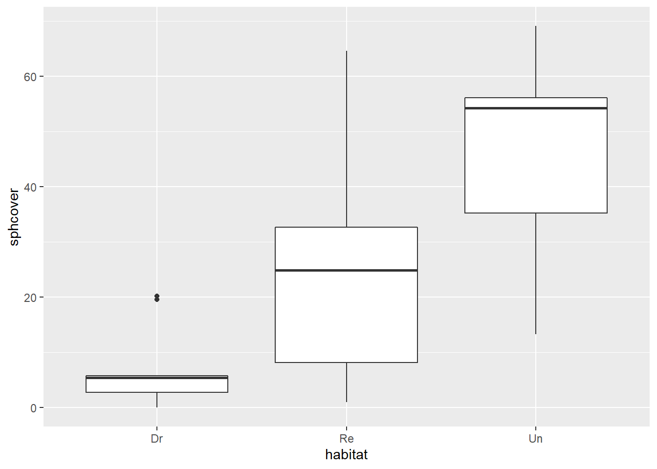

What are the assumptions of a classical ANOVA model that would describe sphagnum moss cover by habitat type? Do these assumptions appear to be met here?

Solution

The ANOVA assumes that the residuals follow a normal distribution of the same variance for each group. Here, the distributions are skewed and the variance seems smaller for the Dr group seems than the others.

Fit the sphcover ~ habitat linear model to the cover dataset. See the summary of the model results with the summary function and the confidence intervals of the coefficients with the confint function. What is the interpretation of each coefficient? Are the confidence intervals plausible?

Solution

mod <- lm(sphcover ~ habitat, data = cover)
summary(mod)

## 
## Call:
## lm(formula = sphcover ~ habitat, data = cover)
## 
## Residuals:
##     Min      1Q  Median      3Q     Max 
## -33.144  -8.161  -0.596   9.659  41.371 
## 
## Coefficients:
##             Estimate Std. Error t value Pr(>|t|)    
## (Intercept)    7.162      5.129   1.396   0.1719    
## habitatRe     16.141      6.282   2.569   0.0149 *  
## habitatUn     39.266      7.254   5.413 5.45e-06 ***
## ---
## Signif. codes:  0 '***' 0.001 '**' 0.01 '*' 0.05 '.' 0.1 ' ' 1
## 
## Residual standard error: 15.39 on 33 degrees of freedom
## Multiple R-squared:  0.4742, Adjusted R-squared:  0.4424 
## F-statistic: 14.88 on 2 and 33 DF,  p-value: 2.473e-05

The intercept is the mean cover for the reference group (drained swamps, Dr). The coefficient habitatRe (respectively, habitatUn) is the difference between the mean cover of rewetted and drained swamps (respectively, the difference between undrained and drained swamps).

confint(mod)

##                 2.5 %   97.5 %
## (Intercept) -3.273495 17.59807
## habitatRe    3.360128 28.92248
## habitatUn   24.507522 54.02438

The confidence interval for the mean of the Dr group reaches negative values, which is not possible for a percentage cover.

Create a function with arguments x and i, which fits the linear model in b) by replacing the original data set (data = cover) with data = x[i, ], and then returns the coefficients of the model with the function coef. Then, apply boot to the cover dataset with the function created and perform 10,000 replicates.

Notes

When the first argument of `boot’ is a dataset, it is the rows of that dataset that are resampled.
Since the statistic calculated by the function has several values (each of the coefficients), the t element of the boot result is a matrix rather than a vector. The columns of this matrix correspond to each of the coefficients in order. You can calculate a statistic for each column with the function apply, e.g. apply(res$t, 2, mean). Here, 2 indicates to calculate the mean function per column (1 would mean per row).

Solution

lm_hab <- function(x, i)  {
    mod <- lm(sphcover ~ habitat, x[i,])
    coef(mod)
}

boot_hab <- boot(cover, lm_hab, R = 10000)

# Mean
apply(boot_hab$t, 2, mean)

## [1]  7.193903 16.132949 39.288069

# Standard error
apply(boot_hab$t, 2, sd)

## [1] 2.529526 4.599182 6.523183

The mean of the bootstrap is very close to the coefficients estimated in b), but the standard errors have decreased.

Note that all coefficients depend on the mean of the reference group Dr. The mean and standard deviation of this group are strongly affected by two extreme values around 20, as shown in graph a). These extreme values will be absent in several bootstrap samples, which has the effect of reducing the estimated standard deviation for the Dr group and thus reducing the standard error of the model’s coefficients.

The application of the bootstrap in c) resamples across all rows, so that the number of observations in each habitat type varies from sample to sample. If it is preferable to consider these numbers as fixed quantities, habitat types can be defined as strata by adding the argument strata = as.factor(cover$habitat) to the boot function. (The conversion of the variable habitat to a factor is necessary here.)

Repeat the analysis in c) with stratified resampling and compare the standard errors obtained for each coefficient.

Solution

boot_strat <- boot(cover, lm_hab, R = 10000, strata = as.factor(cover$habitat))

# Mean
apply(boot_strat$t, 2, mean)

## [1]  7.165948 16.180594 39.323302

# Standard error
apply(boot_strat$t, 2, sd)

## [1] 2.372362 4.490822 6.173863

All standard errors have decreased compared to c).

Calculate the confidence interval for the habitatUn coefficient according to the result of the bootstrap in d). Note that you need to add the argument index = 3 to the function boot.ci to tell R to calculate the interval for the 3rd coefficient.

Solution

boot.ci(boot_strat, index = 3)

## Warning in boot.ci(boot_strat, index = 3): bootstrap variances needed for
## studentized intervals

## BOOTSTRAP CONFIDENCE INTERVAL CALCULATIONS
## Based on 10000 bootstrap replicates
## 
## CALL : 
## boot.ci(boot.out = boot_strat, index = 3)
## 
## Intervals : 
## Level      Normal              Basic         
## 95%   (27.11, 51.31 )   (27.86, 51.77 )  
## 
## Level     Percentile            BCa          
## 95%   (26.76, 50.68 )   (25.24, 49.55 )  
## Calculations and Intervals on Original Scale

Finally, we will resample the model residuals.

Fit a linear model as in b), then add to the dataset cover a column for the model’s fitted values.
Write a function that creates a new dataset by adding a resampled vector x[i] to the expected values to produce a new response variable, then fits a model with this new response variable to the habitat.
Simulate 10,000 samples with the boot function, using as arguments (1) the residuals vector (residuals) of the model and (2) the function created above. Do not specify strata. Recalculate the mean, standard error and 95% confidence interval of the coefficients.

Is resampling the residuals a good choice for these data?

Solution

mod <- lm(sphcover ~ habitat, data = cover)
cover$fitted <- fitted(mod)

lm_resid <- function(x, i) {
    cover$cover_new <- cover$fitted + x[i]
    mod_new <- lm(cover_new ~ habitat, data = cover)
    coef(mod_new)
}

boot_resid <- boot(residuals(mod), lm_resid, R = 10000)

# Mean
apply(boot_resid$t, 2, mean)

## [1]  7.155993 16.157210 39.340901

# Standard error
apply(boot_resid$t, 2, sd)

## [1] 4.941989 6.059448 6.965119

boot.ci(boot_resid, index = 3)

## Warning in boot.ci(boot_resid, index = 3): bootstrap variances needed for
## studentized intervals

## BOOTSTRAP CONFIDENCE INTERVAL CALCULATIONS
## Based on 10000 bootstrap replicates
## 
## CALL : 
## boot.ci(boot.out = boot_resid, index = 3)
## 
## Intervals : 
## Level      Normal              Basic         
## 95%   (25.54, 52.84 )   (25.71, 52.94 )  
## 
## Level     Percentile            BCa          
## 95%   (25.59, 52.82 )   (25.23, 52.53 )  
## Calculations and Intervals on Original Scale

Resampling of the residuals assumes that the residuals in each group are from the same distribution. In this case, the variances are not homogeneous between groups, so it is preferable to re-sample the observations.

The bootstrap method - Solutions

Data

1. Estimation of mean cover for drained swamps

2. Estimation of differences between habitats